Building an Edge-Aware Cell Mapper for Houdini COPs
Edge-Aware Cell Mapper for Houdini COPs
I recently released my Atlas Mapper on Gumroad. It can generate edge-aware ASCII art, apply procedural hatching, create mosaic effects, and do adaptive cell subdivision. Basically everything you need to turn images into grids of stuff.
The feedback I got was unanimous: “I don’t care about the tool, I want to know how it works.” So, while I continue my failed career as a capitalist, here’s the breakdown of how it actually works.
I’ve been fascinated by ASCII shaders for a while now, especially Acerola’s video “I Tried Turning Games Into Text”, which really stuck with me. The workflow we’ll be following is basically the same, but we’re making some adjustments to fit it into the node-based workflow of COPs. Since Acerola’s video goes through the process in detail, I’ll be focusing on the OpenCL specifics rather than the general algorithm.
The complete workflow will look like this:
- Split the input into equally sized cells
- Create UV textures for each cell
- Calculate the average brightness for each cell
- Offset the UV texture using the brightness
- Sample a character from the atlas based on the brightness
After that, we’ll look at directional edge detection and how to use it to respect edges in the image.
 The complete workflow
Splitting the image into cells
The first step is splitting our input image into equal cells, lets start off by just looking at the code to generate a checker pattern.
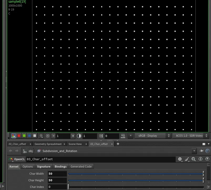
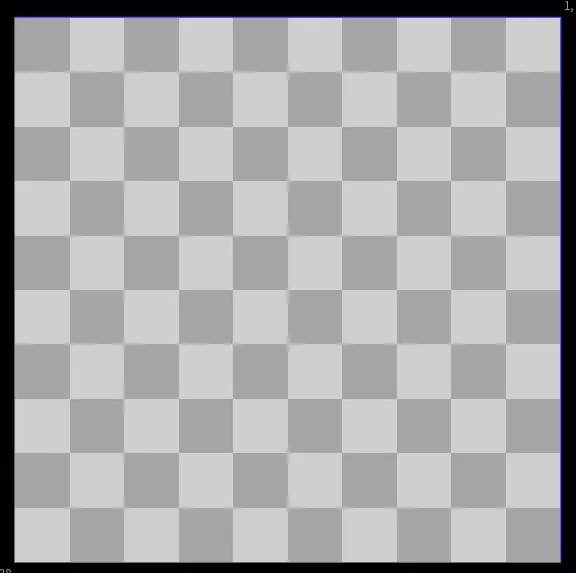 Adjusting Checker size
#bind layer src float4
#bind layer !&output float4
#bind parm char_width int value=50
#bind parm char_height int value=50

@KERNEL
{
int2 gid = (int2)(@ix, @iy);  // Current pixel position

// Which character cell does this pixel belong to?
int2 char_coord = gid / (int2)(@char_width, @char_height);

// Visualize the grid: color cells in checkerboard pattern
float checker = ((char_coord.x + char_coord.y) % 2) == 0 ? 1.0f : 0.5f;
@output.set((float4)(checker, checker, checker, 1.0f));
}
By dividing the pixel coordinates and casting to (int2), we truncate the decimal values, effectively grouping pixels into cell-sized regions. Since we’re working with integer pixel coordinates (@ix, @iy) ranging from 0 to screen width/height, a simple division gives us our cell grid indices.
For example, with a 500×500 image and a cell size of 50 pixels:
- Pixels 0-49 → cell 0
- Pixels 50-99 → cell 1
- Pixels 100-149 → cell 2
and so on, creating a 10×10 grid of cells (0-9 in each dimension)
Note: For clean cell divisions, ensure your image resolution is evenly divisible by your cell size (500 ÷ 50 = 10). Non-divisible resolutions will create partial cells at the edges.
The modulo operator % creates our checkerboard visualization - alternating between 1.0 (white) and 0.5 (gray) based on whether the sum of the cell coordinates is even or odd.
From Grid to UV Coordinates
The checkerboard pattern proves our cell grid is working correctly, each cell is being treated as a single unit. But a simple binary pattern isn’t very useful. What we really need is a way to map each cell to a specific location in our atlas texture. This is where UV coordinates come in. Instead of coloring cells uniformly, we need to generate coordinates that:
- Repeat identically for every cell - so they all can access the same atlas structure
- Can be offset to point at different characters in the atlas based on content
- Preserve pixel position within each cell for proper character rendering
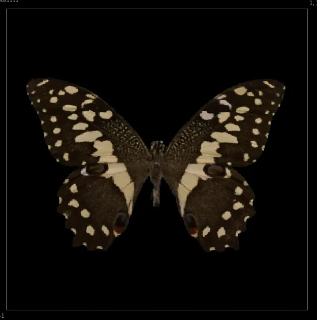
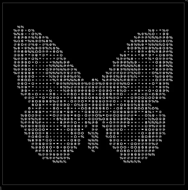
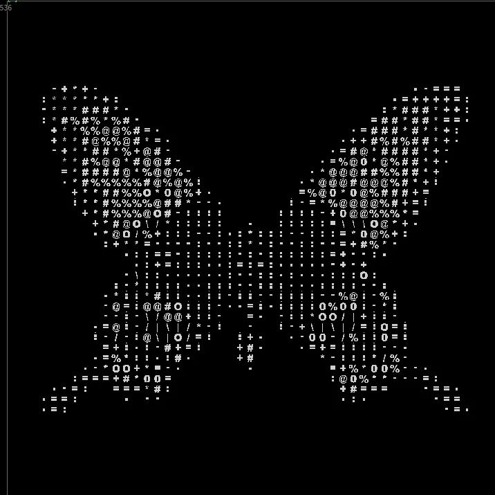
 Adjusting Checker size and Sampling butterfly.pic
int2 gid = (int2)(@ix, @iy); // Current pixel position
// === STEP 1: Determine which cell this pixel belongs to ===
int2 char_coord = gid / (int2)(@char_width, @char_height);
// === STEP 2: Position within the cell (0 to width-1, 0 to height-1) ===
int2 pixel_in_cell = gid % (int2)(@char_width, @char_height);
// === STEP 3: Normalize to 0-1 range within cell ===
// This creates UVs that go from 0.0 at cell start to 1.0 at cell end
float u = (float)pixel_in_cell.x / (float)@char_width;
float v = (float)pixel_in_cell.y / (float)@char_height;
// === STEP 4: Remap to -1 to +1 range (required for UV sampling) ===
// Houdini's UV sample node expects coordinates in -1 to +1 space
// -1 = left/bottom edge, 0 = center, +1 = right/top edge
float u_centered = (u - 0.5f) * 2.0f;
float v_centered = (v - 0.5f) * 2.0f;
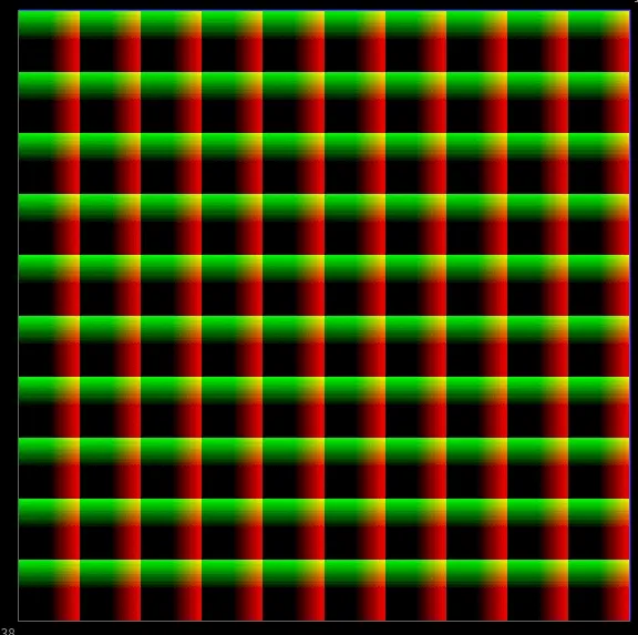
// === OUTPUT: Visualize UVs as colors ===
// Red channel = U (horizontal position in cell)
// Green channel = V (vertical position in cell)
// Each cell now has identical UV gradient from (-1,-1) to (+1,+1)
@output.set((float4)(u_centered, v_centered, 0.0f, 1.0f));
Breaking down the UV generation:
The modulo operator (%) gives us the pixel’s position within its cell, a value from 0 to char_width-1 horizontally and 0 to char_height-1 vertically.
Dividing by the cell dimensions normalizes this to the 0-1 range, creating UVs that reset for every cell.
The centering step (remapping to -1 to +1) is needed because the "UV Sample" Node expects UVs from -1 to 1. Every cell now contains an identical UV coordinate system, ready to be offset to point at different characters in our atlas.
Mapping to Atlas UVs
Now that we have per-cell UVs (0-1 range), we need to offset them to point at specific characters in our atlas texture. The atlas is organized as a grid - for example, a 4x4 grid containing our character ramp: .:-=+*#%@
Given a character index (0-9 for our ramp), we need to convert it to a 2D position in the atlas grid:
// Atlas size (4x4)
int atlas_size = 4;


// === STEP 1: Convert linear character index to 2D grid position ===
int atlas_char_x = @char_index % atlas_size;
int atlas_char_y = @char_index / atlas_size;

// flip the y axis, to start sampling from the top
int flipped_char_y = (atlas_size - 1) - atlas_char_y;

// Normalize pixel position within cell (0-1)
float u = (float)pixel_in_cell.x / (float)@char_width;
float v = (float)pixel_in_cell.y / (float)@char_height;

// === STEP 2: Calculate UV coordinates within the atlas ===
float atlas_u = ((float)atlas_char_x + u) / (float)atlas_size;
float atlas_v = ((float)flipped_char_y + v) / (float)atlas_size;


// === STEP 3: Remap from 0-1 space to -1 to +1 space ===
atlas_u = (atlas_u - 0.5f) * 2.0f;
atlas_v = (atlas_v - 0.5f) * 2.0f;

@output.set((float4)(atlas_u,atlas_v, 0.0f, 1.0f));
We convert the linear character index into a 2D grid position (row and column) within the atlas. The Y-axis is flipped so that index 0 starts at the top of the atlas rather than the bottom. Next, we normalize the pixel’s position within its cell to 0-1 range, then add this to the character’s atlas position and divide by the atlas size—compressing the entire atlas into 0-1 UV space where each character occupies its proportional tile. Finally, we remap from 0-1 to -1 to +1 because Houdini’s UV Sample node expects coordinates in that range.
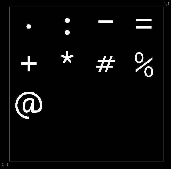 The character atlas texture
 offsetting all of the uv coordinates
Extracting the Average Luminance
 Mapping based on average cell luminance
Next we need to calculate a value to offset the UVs, sampling luminance. Calculating the cell-offset is quite simple and admittedly inefficient by traditional standards. To decide which character to use for each cell, we need to analyze its content—typically its average brightness. We do this by looping through every pixel in the cell and averaging its brightness, but since each pixel needs to have the same value they all loop through the same pixels of each cell. The “redundant” loop:
// Calculate top-left corner of this cell
int2 cell_start = char_coord * (int2)(@char_width, @char_height);

float avg_lum = 0.0f;
int samples = 0;

for (int dy = 0; dy < @char_height; dy++) {
    for (int dx = 0; dx < @char_width; dx++) {
        int2 p = cell_start + (int2)(dx, dy);

        // Bounds check
        if (p.x >= @src.xres || p.y >= @src.yres) continue;

        // Sample and accumulate luminance
        float4 c = (float4)(@src.bufferIndex(p));
        avg_lum += dot(c.xyz, (float3)(0.299f, 0.587f, 0.114f));
        samples++;
    }
}

avg_lum /= (float)samples;
In an 20x20 cell (400 pixels) each pixel independently loops through the same 400 pixels and arrives at the same avg_lum value. While this could be considered wasteful, GPUs thrive on parallel, uniform work. Having all threads execute the same operations in lockstep is faster than trying to coordinate which thread should do the analysis.
One massive performance improvement you can do is use the Layer Tile Size option to run over smaller chunks of the image at a time, or downsample the image beforehand. This way you can avoid the redundant work by having each thread analyze a different chunk of the image. But this only works for square character cells. Since I wanted to keep the flexibility of non-square cells and the performance impact is minimal, I stuck with the redundant work approach.
Adding Intelligence: Edge Detection
So far, we’ve mapped cells based purely on brightness. Dark areas get (space), bright areas get @. This already has a quite cool effect but it can be quite difficult to read some images.
To improve upon that lets now see how to extract edge information from the image, to match cells with high edge values to characters that better represent them.
A vertical edge should map to |, a horizontal edge to -, and diagonals to / or \.
For this, we need to detect not just where edges are, but which direction they run. This requires four separate gradient calculations, one for each major direction.
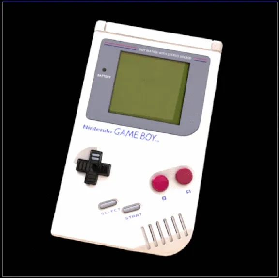
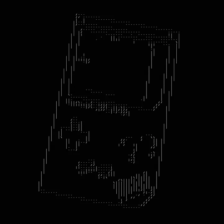 Gameboy with only ASCII edges
The Sobel Operators
Sobel operators are 3×3 convolution kernels that approximate image gradients. A gradient measures how quickly brightness changes in a given direction. High gradient = edge. The genius of Sobel is using perpendicular detection: the horizontal gradient (Gx) detects vertical edges. When brightness changes left-to-right, you’ve found a vertical boundary.
 Input -> Directional edges -> single channels
// Sample 3x3 neighborhood luminance values
float lum[3][3];
for (int dy = -1; dy <= 1; dy++) {
    for (int dx = -1; dx <= 1; dx++) {
        int2 p = gid + (int2)(dx, dy);
        float4 c = (float4)(@src.bufferIndex(p));
        lum[dy+1][dx+1] = dot(c.xyz, (float3)(0.299f, 0.587f, 0.114f));
    }
}

    // Sobel Gx - detects VERTICAL edges (horizontal gradient)
    // Kernel:  -1  0  +1
    //          -2  0  +2
    //          -1  0  +1
    float gx = -lum[0][0] + lum[0][2]
               -2.0f*lum[1][0] + 2.0f*lum[1][2]
               -lum[2][0] + lum[2][2];

    // Sobel Gy - detects HORIZONTAL edges (vertical gradient)
    // Kernel:  -1 -2 -1
    //           0  0  0
    //          +1 +2 +1
    float gy = -lum[0][0] - 2.0f*lum[0][1] - lum[0][2]
               +lum[2][0] + 2.0f*lum[2][1] + lum[2][2];

    // Diagonal / - bottom-left to top-right
    // Kernel:   0 -1 -2
    //          +1  0 -1
    //          +2 +1  0
    float gd1 = -lum[0][1] - 2.0f*lum[0][2] - lum[1][2]
                +lum[1][0] + 2.0f*lum[2][0] + lum[2][1];

    // Diagonal \ - top-left to bottom-right
    // Kernel:  -2 -1  0
    //          -1  0 +1
    //           0 +1 +2
    float gd2 = -lum[0][0] - 2.0f*lum[0][1] - lum[1][0]
                +lum[1][2] + 2.0f*lum[2][1] + lum[2][2];


// Store all four gradients
@edges.set((float4)(gx, gy, gd1, gd2));
Notice we store all four gradients without combining them: (gx, gy, gd1, gd2). This is crucial. Computing edge magnitude sqrt(gx² + gy²) would tell us edge strength, but lose direction information. We need to preserve all four directions separately so we can later determine which is strongest.
Character Selection Logic
With both brightness and edge information available, we can make intelligent character choices:
 Input -> Directional edges -> single channels
 for (int dy = 0; dy < @char_height; dy++) {
        for (int dx = 0; dx < @char_width; dx++) {
            int2 p = cell_start + (int2)(dx, dy);
            if (p.x >= @src.xres || p.y >= @src.yres) continue;

            float4 c = (float4)(@src.bufferIndex(p));
            avg_lum += dot(c.xyz, (float3)(0.299f, 0.587f, 0.114f));

            float4 e = (float4)(@edges.bufferIndex(p));
            max_edges = max(max_edges, fabs(e));

            samples++;
        }
    }

    avg_lum /= (float)samples;

    // Find strongest edge
    float max_edge_strength = max(max(max_edges.x, max_edges.y),
                                   max(max_edges.z, max_edges.w));
Since we’re looping through the cell, to sample luminance we can also keep track of the strongest edge direction.
Edge gradients can be positive or negative depending on which direction is brighter: Positive gx, bright on right, dark on left. Negative gx, dark on right, bright on left
But both represent the same vertical edge, just with inverted contrast. We use fabs() (absolute value) because we only care about edge strength, not polarity.
After the Loop we extract the strongest direction using nested max() functions.
    // === SELECT CHARACTER ===
    int char_index = 0;

    if (max_edge_strength > @edge_threshold) {
        if (max_edges.x == max_edge_strength) {
            char_index = 0;
        } else if (max_edges.y == max_edge_strength) {
            char_index = 1;
        } else if (max_edges.z == max_edge_strength) {
            char_index = 2;
        } else {
            char_index = 3;
        }
    } else {
        // characters "|-/\ .:-=+*#%@0O"
        // offset the luminance by 4 characters to fit the edge values at the start
        char_index = (int)(clamp(avg_lum, 0.0f, 0.999f) * 10.0f + 4.0f);
    }
Now we bring it all together. For each cell, we have:
- Average brightness (
avg_lum) - Maximum edge strength in four directions (
max_edges)
The decision logic is simple: if any edge is strong enough (above threshold), use a directional character. Otherwise, fall back to brightness-based selection.
This gives us ASCII art that preserves both the tonal values (light/dark) and structural information (edges and their orientations) of the original image.
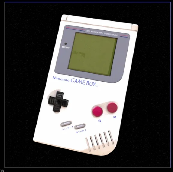
 Animated Edge Threshold
That’s it! You can adapt this to make a lot of cool things since we’re just sampling a texture. hatching patterns, mosaic tiles or output the cell luminance values and feed them through a color ramp for stylized tinting.
Download
If you want to support my work, you can buy the tool on Gumroad where you will also find the free files for this blog post.
The paid version extends everything covered here and more! It also adds:
- Adaptive subdivision (variance-based cell sizing)
- UV rotation (random, mapping-based, or layer-driven) Which enables sweet truchet tiles
- 13 mapping modes (hue, saturation, RGB channels, warmth)
- Pre-built atlas generators for ASCII characters and SOP-based shapes
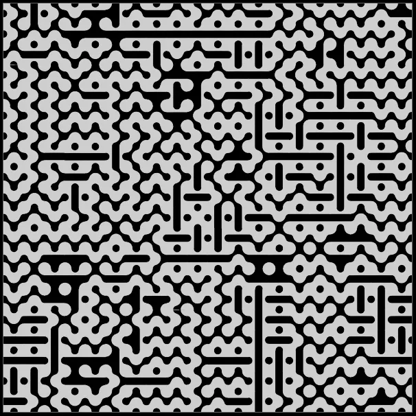 Rotation and Adaptive Subdivision
Sources and Links
- Acerola’s Video “I Tried Turning Games Into Text”
- Alex Harri “ASCII Rendering” — an insanely detailed breakdown of the topic, which I only found after finishing the tool.